Reaction Diffusion
Natural pattern simulation using the Gray Scott algorithm with WebGL, with a interactive simulation at the end.
Reaction Diffusion
One of the most beautiful fields of science lies between biology and computer science. With just a couple of simple rules inspired by nature, it is possible to create the most complex systems. Examples of these are flocking behaviors, Lindenmayer-systems and slime-mold networks. However, in this blog post I want to focus on another system: Reaction diffusion systems. Reaction diffusion systems are systems that are known to create all kinds of patterns that can be found in nature, like stripes on a zebra, or spots on a giraffe. And actually these patterns are also sometimes known as Turing patterns, named after Alan Turing, who is not only the father of the theory of computation, but also wrote one of the foundational papers about how these patterns can arise seemingly by itself in nature.
 A reaction diffusion system is a system which describes the concentrations of specific particles or
chemicals in space. In these systems there are two mayor dynamics that are happening: reaction and diffusion.
There is a reaction of some kind, between the different kind of chemicals. And besides that there is
diffusion happening of these chemicals though the space. If we for example have a 2 dimensional space with
two kinds of chemicals A and B, the reaction diffusion system can generate all kinds of patterns by the
interaction between the reaction that is happening between chemical A and B and the diffusion of these
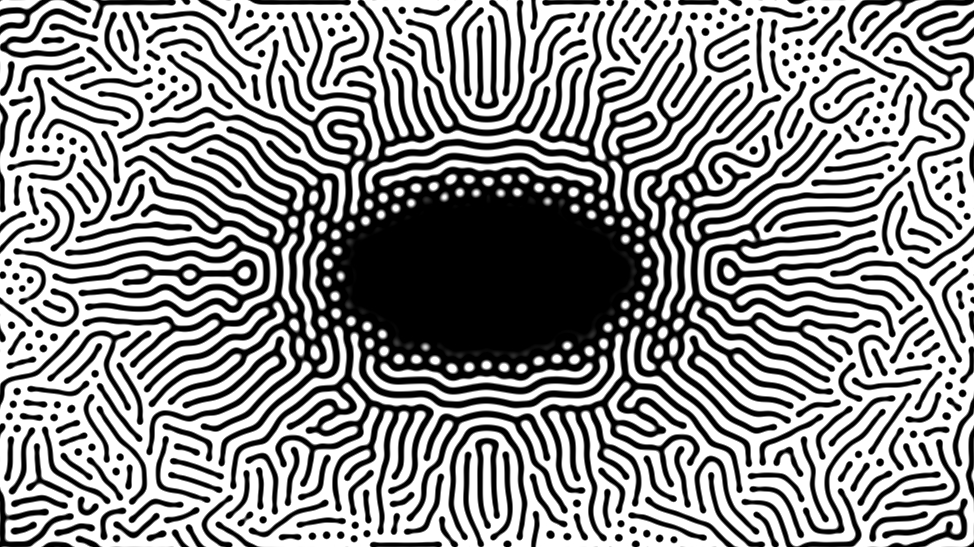
two chemicals. Because of this we can get waves of concentrations gradients which flow through the two
dimensional space. These waves we then can visualise, and get patterns like you see on the
left image.
A reaction diffusion system is a system which describes the concentrations of specific particles or
chemicals in space. In these systems there are two mayor dynamics that are happening: reaction and diffusion.
There is a reaction of some kind, between the different kind of chemicals. And besides that there is
diffusion happening of these chemicals though the space. If we for example have a 2 dimensional space with
two kinds of chemicals A and B, the reaction diffusion system can generate all kinds of patterns by the
interaction between the reaction that is happening between chemical A and B and the diffusion of these
two chemicals. Because of this we can get waves of concentrations gradients which flow through the two
dimensional space. These waves we then can visualise, and get patterns like you see on the
left image.
Gray Scott Algorithm
One of these reaction diffusion algorithms is the Gray-Scott algorithm. This algorithm is a reaction between chemical $A$ and chemical $B$, where two particles of chemical $B$ plus a particle of chemical $A$ change into 2 particles of chemical $B$ The formulas for the change of concentration of both chemicals are described below. We can see for the new concentrations of $A$ and $B$ we take the previous concentrations plus the change in concentration times the time step $dt$. The change in the chemicals for both $A$ and $B$ is described by 3 factors. Let's go through them one by one.
Diffusion
The first is the diffusion factor. The diffusion factor $D_A \Delta A$ containst first of all a diffusion rate $D_A$, which is a specific constant for the chemical. But more interestingly we multiply this by $\Delta A_t$, which is the Laplacian of the concentration of $A$ at time $t$ (the second positional derivative of the amount of chemical $A$). This Laplacian is key to the diffusion part of the algorithm. The Laplacian encodes the difference in concentration between the point we want to calculate, and the surrounding points. This is good because the diffusion should change the amount of $A$ in such a way that it flows from high concentrations to lower concentrations. This part of the equation is actually similar to the heat equation. In practice, when coding the Laplacian, we do not solve the Laplacian analytically though, we actually use a convolutional kernel which encodes this Laplacian operator at every timestep.
Reaction
Besides the diffusion we have the reaction. The reaction between $A$ and $B$ can be found in the formulas as the term $A*B^2$. We also see that this term is removed from $A$, but added to $B$. Is encodes the particles of $A$ that change into $B$. The rate of this reaction is proportional to A, because when there are more particles of A, the reaction has more change to happen and the speed of the reaction increases. This reasoning can also be applied to the concentration of $B$, but $B$ is used 2 times in the reaction. Therefore reaction speed is actually related to $B^2$, which then results in the reaction term.
Feed and kill rates
 And finally we have the last terms in both the reactions. These are the feed and kill rate.
One can imagine that when we have particles of $A$ reacting to particles of $B$,
we finally end up with only $B$ everywhere. To sustain the reaction, there is a feed rate and a kill rate.
The feed rate replenishes $A$, and the kill rate reduces $B$. We can let the pattern generation start
by starting with a 2 dimensional canvas which is full of chemical $A$ and has no $B$,
we then seed it at some place with chemical $B$, and the pattern starts growing.
And finally we have the last terms in both the reactions. These are the feed and kill rate.
One can imagine that when we have particles of $A$ reacting to particles of $B$,
we finally end up with only $B$ everywhere. To sustain the reaction, there is a feed rate and a kill rate.
The feed rate replenishes $A$, and the kill rate reduces $B$. We can let the pattern generation start
by starting with a 2 dimensional canvas which is full of chemical $A$ and has no $B$,
we then seed it at some place with chemical $B$, and the pattern starts growing.
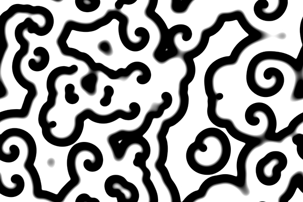
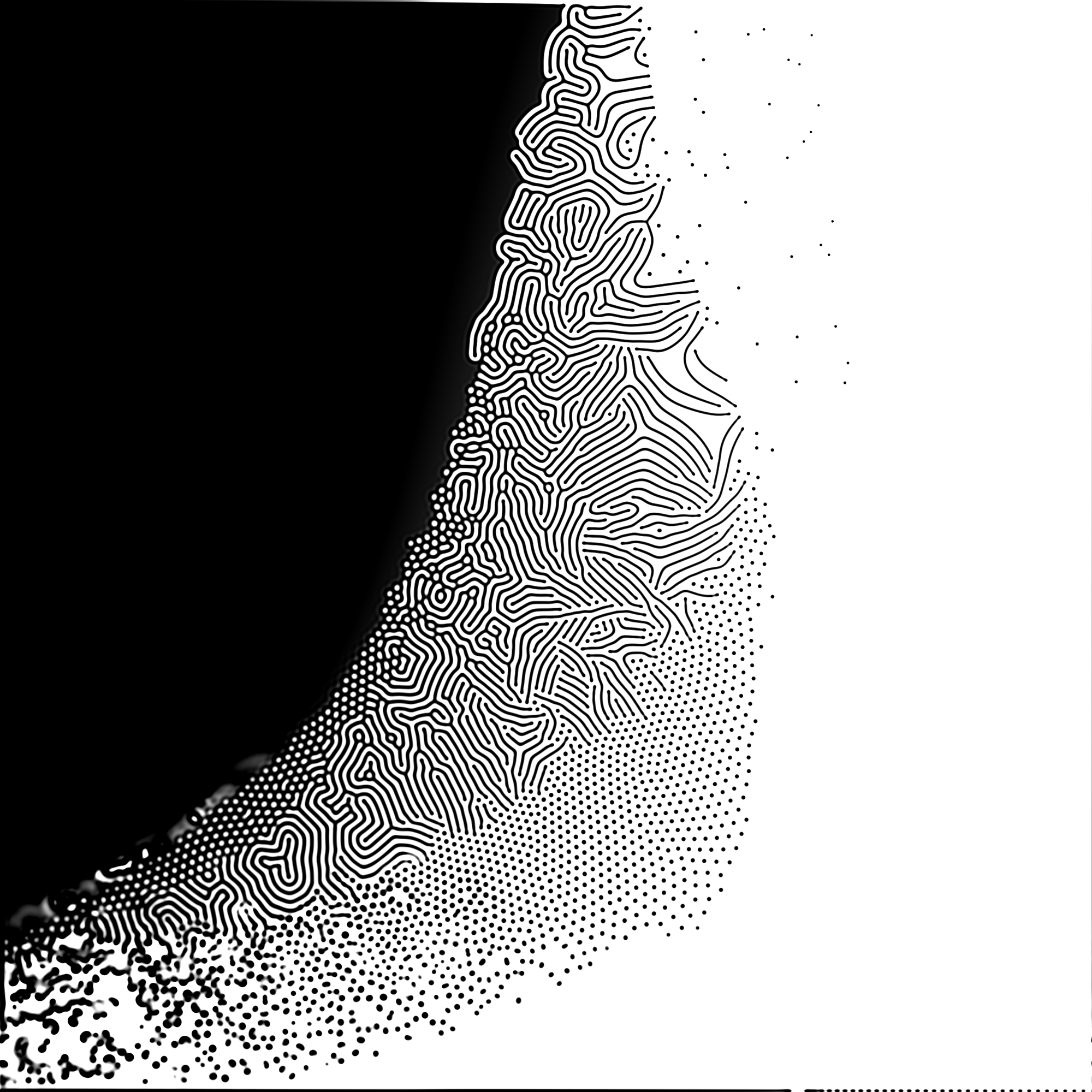
What kind of patterns are the result of the algorithm are based on that numbers you choose for the constants in the formulas ($D_A$, $D_B$, $f$ and $k$). By changing the feed and kill rate the patterns change from spirals, to worms, to blobs. You can see how the feedrate and killrate have effect on the pattern in the image on the right, which changes in feedrate on the y-axis, and in kullrate on the x-axis. You can play with a interactive simulation of this a bit in the image at the end of the page, where you can change the feed rate with the slider underneath. Besides that there is a kill rate gradient in the simulation going from left to right.
Three.js and WebGL
One can simulate this algorithm easily in several languages and packages. For example Daniel Shiffman has a very nice tutorial on how to do this on YouTube in p5.js. However, when you want to run this simulation at faster speeds, you would want to accelerate it on a GPU, which is much faster in these parallel computations like the Laplacian kernel. Because of this I implemented the simulations you can see above and below using the THREE.js library and some GLSL script, such that it can run using WebGL. This is the first time I do a project with JavaScript, THREE.js and WebGL. Is has been great fun to learn how to do CPU acceleration for in the browser. The resulting simulations are quite fun and fast enough to keep playing with them. If you want to check out how I did this or play more with the algorithm, you can check out the repo on GitHub.